|
|
![]()
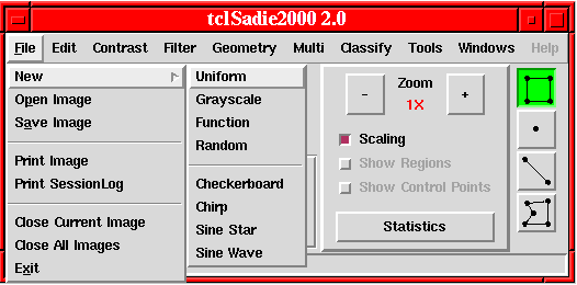
Click on the File > New > Image Type above to see function information.
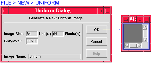
Creates an image with a uniform graylevel across the entire image. Size of image is given in lines (rows) and pixels (columns).
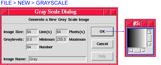
The Grayscale command creates a horizontal grayscale gradient pattern. Parameters are the size of the image to be generated, the minimum and the maximum graylevel values, and the number of distinct graylevels. The generated grayscale has the minimum graylevel on the left, and the maximum graylevel on the right side.
The Geometry > Rotate command may be used to reverse the order of graylevels in the output image, or to rotate the grayscale from horizontal to vertical.
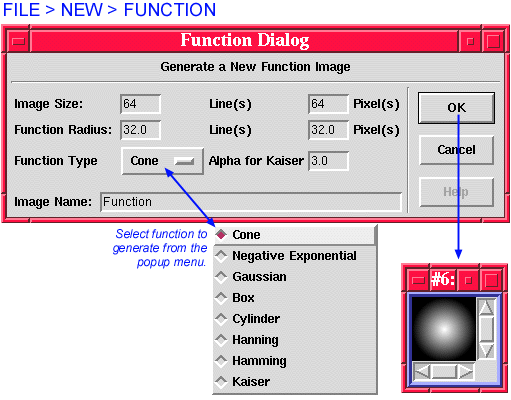
The Function command generates a variety of two-dimensional test functions. Parameters are the size of the generated image, the function’s radii, and the function type, selected from a pop-up menu on the dialog.
The graylevel value of a pixel in the output image O at coordinates (j,k) is computed for the various types of test functions as
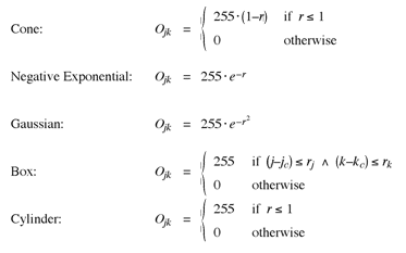
where r is the radius and j/k and jc/kc are the coordinates of the given point and the center, respectively, and e is the base of the natural logarithm (i.e., e = ln(1) = 2.718282…).
The Hanning, Hamming, and Kaiser functions are 1D functions applied with circular symmetry to create a 2D image:
Hanning Window
![]()
Hamming Window
![]()
Kaiser Window
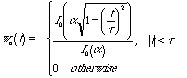
where,
The continuous 1D variable ![]() , n1 and n2 are lines and pixels/line in the 2D image, and
, n1 and n2 are lines and pixels/line in the 2D image, and ![]() is the period of the image. I0 ( ) is the zeroth-order modified Bessel function of the first
kind.
is the period of the image. I0 ( ) is the zeroth-order modified Bessel function of the first
kind.
The generated image can be subsequently used as a kernel in a Filter > Convolution or Filter > FFT Convolution command.
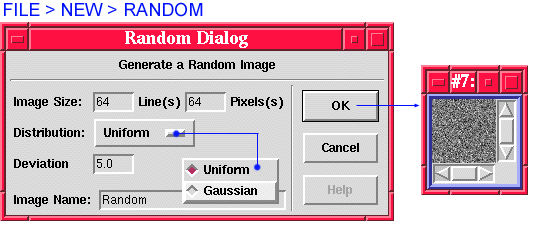
The Random command creates an image consisting of a pseudo-random pattern. Parameters are the size of the image to be generated, the probability distribution of the image’s graylevel values, and the graylevel deviation, which corresponds to either the range (in the case of a uniform distribution) or the standard deviation (in the case of a gaussian distribution). The graylevel distribution is chosen from a pop-up menu.
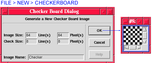
The Checkerboard command generates a binary checkerboard pattern, starting with a black rectangle (a graylevel of 0) in the upper left corner, and alternating between white and black (graylevels of 255 and 0, respectively) thereafter. Parameters are the number of lines and the number of pixels per line of the output image, and the vertical and horizontal extent of an individual rectangle.
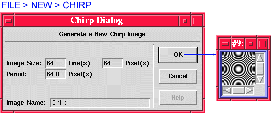
The Chirp function generates an exponentially decaying sine function with a given period.
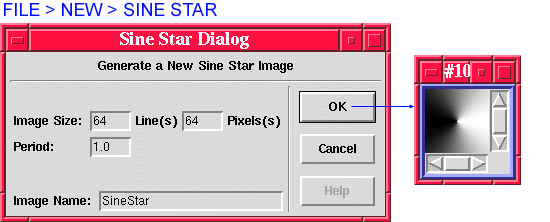
The Sine Star function generates an image where the grey levels at a specific radius from the center follow a sine function along the circumference of the circle.
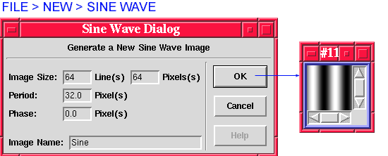
The Sine Wave command creates a horizontal sinewave pattern. Parameters are the size of the output image, and the period and phase of the sinewave. Cosine wave patterns may be generated easily by setting the phase to one-fourth of the period (pixels). Geometry > Rotate may be used to rotate the pattern to any angle.
Last Updated: August 2000
University of Arizona
Electrical and Computer Engineering Department
Digital Image Analysis Laboratory © 1999,2000